为何实现一个BP神经网络?
“What I cannot create, I do not understand”
— Richard Feynman, February 1988
实现一个BP神经网络的7个步骤
选择神经网络 结构
随机 初始化权重实现 前向传播
实现 成本函数 $J(\Theta)$
实现反向传播算法并计算 偏微分 $\frac{\partial}{\partial
使用 梯度检查 并在检查后关闭
使用梯度下降或其它优化算法和反向传播来 优化 $\Theta$ 的函数 $J(\Theta)$
数据集 我们选取著名的鸢尾花数据集作为神经网络作用的对象,首先先观察下数据。
1 2 3 4 5 6 7 8 9 10 11 12 13 14 15 16 17 In[2 ]: import numpy as npfrom sklearn import datasetsiris = datasets.load_iris() perm = np.random.permutation(iris.target.size) iris.data = iris.data[perm] iris.target = iris.target[perm] print iris.data.shapeprint iris.target.shape np.unique(iris.target) Out[2 ]: (150 , 4 ) (150 ,) array([0 , 1 , 2 ])
可见,鸢尾花数据集有四个特征,分为三种类别,总共150个条数据。
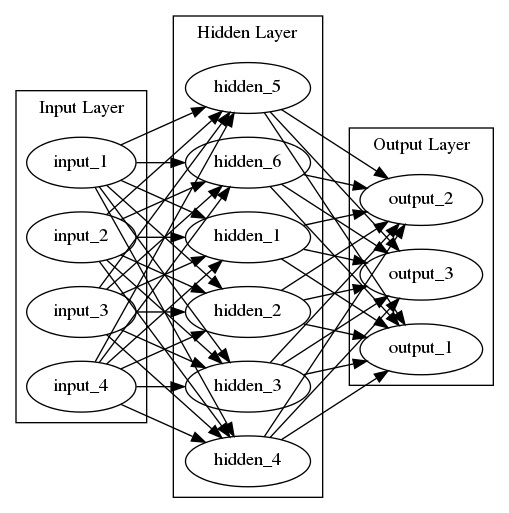
选择人工神经网络结构
随机初始化权重 网络权重随机初始化 初始化 $\Theta_{ij}^{(l)}$ 为 $[-\epsilon, \epsilon]$ 之间的随机值。
初始化函数可定义如下:
1 2 3 4 5 In[3 ]: def random_init (input_layer_size, hidden_layer_size, classes, init_epsilon=0.12 ) : Theta_1 = np.random.rand(hidden_layer_size, input_layer_size + 1 ) * 2 * init_epsilon -init_epsilon Theta_2 = np.random.rand(classes, hidden_layer_size + 1 ) * 2 * init_epsilon -init_epsilon return (Theta_1, Theta_2)
实现前向传播 每一层都以此为公式计算下一层:
$$
注意添加偏差项。
前向传播函数定义如下 1 2 3 4 5 6 7 8 9 In[4 ]: def g (theta, X) : return 1 / (1 + np.e ** (-np.dot(X, np.transpose(theta)))) def predict (Theta_1, Theta_2, X) : h = g(Theta_1, np.hstack((np.ones((X.shape[0 ], 1 )), X))) o = g(Theta_2, np.hstack((np.ones((h.shape[0 ], 1 )), h))) return o
实现成本函数 成本函数的数学表示 $${i=1}^m {k=1}^Kyk^{(i)}\log(h \Theta(x^{(i)}))_k + (1 -k^{(i)})\log(1-h \Theta(x^{(i)}))k)] + \frac{\lambda}{2m}\sum {l=1}^{L-1}\suml}\sum {j=1}^{s{l+1}}(\Theta {ji}^{(l)})^2
$K$是输出层单元个数, $L$是层数,我们这里是三, $s_l$ 是层 $l$ 中单元数。
1 2 3 4 5 6 7 8 9 10 11 12 13 14 15 16 17 In[5 ]: def costfunction (nn_param, input_layer_size, hidden_layer_size, classes, X, y, lamb_da) : Theta_1 = nn_param[:hidden_layer_size * (input_layer_size + 1 )].reshape((hidden_layer_size, (input_layer_size + 1 ))) Theta_2 = nn_param[hidden_layer_size * (input_layer_size + 1 ):].reshape((classes, (hidden_layer_size + 1 ))) m = X.shape[0 ] y_recoded = np.eye(classes)[y,:] regularator = (np.sum(Theta_1**2 ) + np.sum(Theta_2 ** 2 )) * (lamb_da/(2 *m)) a3 = predict(Theta_1, Theta_2, X) J = 1.0 / m * np.sum(-1 * y_recoded * np.log(a3)-(1 -y_recoded) * np.log(1 -a3)) + regularator return J
因为scipy中优化函数要求输入参数是向量而不是矩阵,因此我们的函数实现也必须能够随时展开和复原矩阵。
实现反向传播
正向传播计算网络输出
反向计算每一层的误差$\sigma^{(l)}$
由误差累加计算得到成本函数的偏微分$\frac{\partial}{\partial\Theta_{ij}^{(l)}}J(\Theta)$
同样,在实现函数时因为要传递给scipy.optimize模块中的优化函数,必须能展开矩阵参数为向量并可随时复原。
详细实现过程参见Andrew NG在Coursera上的讲座。
数学推导过程请 自行 上coursera ml课程论坛搜索。
1 2 3 4 5 6 7 8 9 10 11 12 13 14 15 16 17 18 19 20 21 22 23 24 25 In[6 ]: def Gradient (nn_param, input_layer_size, hidden_layer_size, classes, X, y, lamb_da) : Theta_1 = nn_param[:hidden_layer_size * (input_layer_size + 1 )].reshape((hidden_layer_size, (input_layer_size + 1 ))) Theta_2 = nn_param[hidden_layer_size * (input_layer_size + 1 ):].reshape((classes, (hidden_layer_size + 1 ))) m = X.shape[0 ] Theta1_grad = np.zeros(Theta_1.shape); Theta2_grad = np.zeros(Theta_2.shape); for t in range(m): a1 = np.hstack((np.ones((X[t:t+1 ,:].shape[0 ], 1 )), X[t:t+1 ,:])) a2 = g(Theta_1, a1) a2 = np.hstack((np.ones((a2.shape[0 ], 1 )), a2)) a3 = g(Theta_2, a2) yy = np.zeros((1 , classes)) yy[0 ][y[t]] = 1 delta_3 = a3 - yy;
续上页
1
2
3
4
5
6
7
8
9
10
11
12
13
14
15
16
delta_2 = delta_3.dot(Theta_2) * (a2 * (1 - a2)) delta_2 = delta_2[0 ][1 :] delta_2 = np.transpose(delta_2) delta_2 = delta_2.reshape(1 , (np.size(delta_2))) Theta1_grad = Theta1_grad + np.transpose(delta_2).dot(a1); Theta2_grad = Theta2_grad + np.transpose(delta_3).dot(a2); Theta1_grad = 1.0 / m * Theta1_grad + lamb_da / m * np.hstack((np.zeros((Theta_1.shape[0 ], 1 )), Theta_1[:, 1 :])) Theta2_grad = 1.0 / m * Theta2_grad + lamb_da / m * np.hstack((np.zeros((Theta_2.shape[0 ], 1 )), Theta_2[:, 1 :])) Grad = np.concatenate((Theta1_grad.ravel(), Theta2_grad.ravel()), axis=0 ) return Grad
梯度检测
“But back prop as an algorithm has a lot of details and,you know, can be a
– Andrew NG如是说
即使看上去成本函数在一直减小,可能神经网络还是有问题。
梯度检测能让你确认,哦,我的实现还正常。
梯度检测原理 简单的微分近似。但相比反向传播神经网络算法计算量更大。
$${i}}J(\theta) \approx {i}+\epsilon) - J(\theta_{i}+\epsilon) }{2\epsilon}
这种梯度计算实现如下: 1 2 3 4 5 6 7 8 9 10 11 12 In[7 ]: def compute_grad (theta, input_layer_size, hidden_layer_size, classes, X, y, lamb_da, epsilon=1e-4 ) : n = np.size(theta) gradaproxy = np.zeros(n) for i in range(n): theta_plus = np.copy(theta) theta_plus[i] = theta_plus[i] + epsilon theta_minus = np.copy(theta) theta_minus[i] = theta_minus[i] - epsilon gradaproxy[i] = (costfunction(theta_plus, input_layer_size, hidden_layer_size, classes, X, y, lamb_da) - costfunction(theta_minus, input_layer_size, hidden_layer_size, classes, X, y, lamb_da)) / (2.0 * epsilon) return gradaproxy
把一切放到一起 先定义训练函数如下:
1 2 3 4 5 6 7 8 9 10 11 12 13 14 15 16 In[8 ]: from scipy import optimizedef train (input_layer_size, hidden_layer_size, classes, X, y, lamb_da) : Theta_1, Theta_2 = random_init(input_layer_size, hidden_layer_size, classes, init_epsilon=0.12 ) nn_param = np.concatenate((Theta_1.ravel(), Theta_2.ravel())) final_nn = optimize.fmin_cg(costfunction, np.concatenate((Theta_1.ravel(), Theta_2.ravel()), axis=0 ), fprime=Gradient, args=(input_layer_size, hidden_layer_size, classes, X, y, lamb_da)) return final_nn
使用训练集进行训练 我选取鸢尾花数据集的100条作为训练集,剩下50条作为测试集。
1 2 3 4 5 6 7 8 9 10 11 12 13 14 15 In[9 ]: X = iris.data[:100 ] y = iris.target[:100 ] lamb_da = 1.0 input_layer_size = 4 hidden_layer_size = 6 classes = 3 final_nn = train(input_layer_size, hidden_layer_size, classes, X, y, lamb_da) Warning: Desired error not necessarily achieved due to precision loss. Current function value: 0.878999 Iterations: 48 Function evaluations: 152 Gradient evaluations: 140
检测两种方式计算的梯度是否近似 1 2 3 4 5 6 7 8 9 10 11 In[10 ]: grad_aprox = compute_grad(final_nn, input_layer_size, hidden_layer_size, classes, X, y, lamb_da) grad_bp = Gradient(final_nn, input_layer_size, hidden_layer_size, classes, X, y, lamb_da) print (grad_aprox - grad_bp) < 1e-1 [ True True True True True True True True True True True True True True True True True True True True True True True True True True True True True True True True True True True True True True True True True True True True True True True True True True True ]
对测试集使用训练得来的参数 可以看到,测试集中50个样本有_个判定错误,其它_个分类正确。
1 2 3 4 5 6 7 8 9 10 11 12 13 14 15 In[11 ]: def test (final_nn, input_layer_size, hidden_layer_size, classes, X, y, lamb_da) : Theta_1 = final_nn[:hidden_layer_size * (input_layer_size + 1 )].reshape((hidden_layer_size, input_layer_size + 1 )) Theta_2 = final_nn[hidden_layer_size * (input_layer_size + 1 ):].reshape((classes, hidden_layer_size + 1 )) nsuccess = np.sum(np.argmax(predict(Theta_1, Theta_2, X), axis=1 ) == y) return nsuccess n = test(final_nn, input_layer_size, hidden_layer_size, classes, iris.data[100 :], iris.target[100 :], lamb_da) print nn = test(final_nn, input_layer_size, hidden_layer_size, classes, iris.data[:100 ], iris.target[:100 ], lamb_da) print nOut[11 ]: 47 99
另一个例子:手写数字数据集 最后是对同样著名的手写数字数据集的实验。
载入并观察数据集: 1 2 3 4 5 6 7 8 9 10 11 12 13 14 15 In[12 ]: digits = datasets.load_digits() perm = np.random.permutation(digits.target.size) digits.data = digits.data[perm] digits.target = digits.target[perm] print digits.data.shapeprint digits.target.shapeprint np.unique(digits.target)Out[12 ]: (1797 , 64 ) (1797 ,) [0 1 2 3 4 5 6 7 8 9 ]
选择神经网络参数 取1000个样本作为训练集,剩下作为测试集。
1 2 3 4 5 6 7 8 9 10 11 12 13 14 15 16 In[13 ]: X = digits.data[:1000 ] y = digits.target[:1000 ] lamb_da = 1.0 input_layer_size = 64 hidden_layer_size = 10 classes = 10 final_nn = train(input_layer_size, hidden_layer_size, classes, X, y, lamb_da) Out[13 ]: Warning: Desired error not necessarily achieved due to precision loss. Current function value: 0.594474 Iterations: 965 Function evaluations: 2210 Gradient evaluations: 2189
进行梯度检测 1 2 3 4 5 6 7 8 In[14 ]: grad_aprox = compute_grad(final_nn, input_layer_size, hidden_layer_size, classes, X, y, lamb_da) grad_bp = Gradient(final_nn, input_layer_size, hidden_layer_size, classes, X, y, lamb_da) print np.all((grad_aprox - grad_bp) < 1e-1 )Out[14 ]: True
对测试集使用训练得来的参数 1 2 3 4 5 6 7 8 9 10 11 12 In[15 ]: n = test(final_nn, input_layer_size, hidden_layer_size, classes, digits.data[1000 :], digits.target[1000 :], lamb_da) print nn = test(final_nn, input_layer_size, hidden_layer_size, classes, digits.data[:1000 ], digits.target[:1000 ], lamb_da) print nOut[15 ]: 722 991
BY REVERLAND